Classification of landtypes
Pierre-Marie Lefeuvre
2025-04-22
Source:vignettes/classification_landtype.Rmd
classification_landtype.RmdClassification of artificial and vegetation landtypes
Following the WMO
Sources: - Temperature siting classification in Nordic Countries from Met’s 2016 reports
sitingclass
Compute landtype
Getting started
Running the function for a station is as follows:
# Load library
library(sitingclass)
library(ggplot2)
library(tidyterra)
#library(patchwork)

# Get station metadata
stn <- get_metadata_frost(stationid = 18700, dx = 100, resx = 1, path = NULL)
# Set default path to NULL in order to print and not save plots

# Compute land cover
landtype_out <- compute_landtype(stn, f_plot=TRUE)
[1] "Process: 18700 - 260966.8/6652718.0 - dtm - 100/1 - path: data/dem"
[1] "Load demo file: data/dem/18700_dtm_25833_d00100m_1.0m.tif"
[1] "Process: 18700 - 260966.8/6652718.0 - dom - 100/1 - path: data/dem"
[1] "Load demo file: data/dem/18700_dom_25833_d00100m_1.0m.tif"
center
landtype_out class : SpatVector
geometry : polygons
dimensions : 7, 1 (geometries, attributes)
extent : 260865.8, 261067.2, 6652618, 6652819 (xmin, xmax, ymin, ymax)
coord. ref. : ETRS89 / UTM zone 33N (EPSG:25833)
names : landtype
type : <fact>
values : tree
bush
cropIn details
The area of reference or bounding box is set using
make_bbox(stn) but the square bbox is reset using the DEM’s
area after their difference to accommodate for some marginal geometrical
differences such as +/- 1 meter caused by a shift in the reference
corner during the data download and after rounding the station
coordinates.
Eventually, the dimension of the returned DEM difference is extracted (i.e. the number of pixel) as it sets the image resolution that I will obtain from the WMS query in the next part.
# Construct box to extract WMS tile
box <- make_bbox(stn)

# Download DEMs
dem <- download_dem_kartverket(stn, name = "dtm")
[1] "Process: 18700 - 260966.8/6652718.0 - dtm - 100/1 - path: data/dem"
[1] "Load demo file: data/dem/18700_dtm_25833_d00100m_1.0m.tif"
dsm <- download_dem_kartverket(stn, name = "dom")[1] "Process: 18700 - 260966.8/6652718.0 - dom - 100/1 - path: data/dem"
[1] "Load demo file: data/dem/18700_dom_25833_d00100m_1.0m.tif"
# Verify extent match
if( terra::ext(dem) != terra::ext(dsm) ){
print("!! Mismatched extent !!")
print(terra::ext(dem))
print(terra::ext(dsm))
# Reload DEMs
dem <- download_dem_kartverket(stn, name = "dtm", f_overwrite = TRUE)
dsm <- download_dem_kartverket(stn, name = "dom", f_overwrite = TRUE)
}
# Compute difference to assess vegetation
dh <- dsm - dem
# The number of pixels to extract from the WMS
px <- dim(dh)[1] #*4
print(sprintf("Pixel number: %i", px))[1] "Pixel number: 201"Three specific layers are extracted from the FellesKartDatabase (FKB) maintained by Kartverket on their geonorge.no servers. The FKB registers buildings, roads and water bodies for official usage. Access to the vector version of these layers is restricted, therefore the vectors are recreated from the images they provide in their WMS distribution service.
# Load FKB-AR5 tiles
building <- get_tile_wms(box, layer = "bygning", px = px)
road <- get_tile_wms(box, layer = "fkb_samferdsel", px = px)
water <- get_tile_wms(box, layer = "fkb_vann", px = px)
g1 <- ggplot() + geom_spatraster_rgb(data = building) + theme_void()
g2 <- ggplot() + geom_spatraster_rgb(data = road) + theme_void()
g3 <- ggplot() + geom_spatraster_rgb(data = water) + theme_void()
# Load complete/original FKB data
fkb <- get_tile_wms(box, layer = "fkb", px = px)
g0 <- ggplot() + geom_spatraster_rgb(data = fkb) + theme_void()
#patchwork::wrap_plots(g0, g1, g2, g3, ncol=2, nrow=2)The images are then: - converted from rasters to vector using
as.polygons(), - the white background vectors that have a
value of 255 are removed, - the vectors are then given a unique
identifier here id = "building", - the vectors are smoothed
with a buffer of 1/4th the resolution of the raster, so 0.25 m as the
default resolution for the raster is 1 m, - the vectors are then
aggregated into one layer, - and plotted Finally all artificial land
vectors are combined into one as shown in the final plot.
# Convert raster tile to vector landcover
v_building <- raster_to_vector(building,
id = "building",
mask_thr = 255)
v_road <- raster_to_vector(road,
id = "road",
mask_thr = 255)
v_water <- raster_to_vector(water,
id = "water",
mask_thr = 255)
# Combine and plot
landtype_artificial <- terra::vect(c(v_building, v_road, v_water))
ggplot(data = landtype_artificial) +
tidyterra::geom_spatvector(aes(fill = value), linewidth = 0) +
theme_minimal()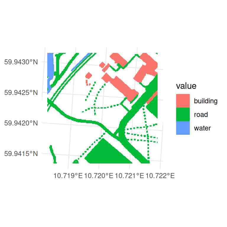
center
To retrieve the vegetation height and its land cover, the DEM
difference dh is used, but first the artificial area are
masked out.
To the masked difference dh_mask, a height threshold is
applied following WMO’s recommendation: - grass: below or equal 10 cm -
crop: between 10 cm and 25 cm - bush: between 25 cm and 3 m - tree:
above and equal to 3 m
# Mask already identified land cover
dh_mask <- terra::mask(dh,
landtype_artificial,
inverse = TRUE,
touches = FALSE)
# Classify vegetation based on dh thresholds in metre
v_grass <- raster_to_vector(dh_mask <= .10,
id = "grass",
mask_thr = FALSE)
v_crop <- raster_to_vector((dh_mask > .10 & dh_mask <= .25),
id = "crop",
mask_thr = FALSE)
v_bush <- raster_to_vector((dh_mask > .25 & dh_mask <= 3),
id = "bush",
mask_thr = FALSE)
v_tree <- raster_to_vector(dh_mask >= 3,
id = "tree",
mask_thr = FALSE)Some work is still required to merge properly the layers together to avoid for instance overlap. After having set each layer a factor level with its name as a label, the overlaps are removed with the priority order set by the order of the factors/levels, such as: 1. “building” 2. “road” 3. “water” 4. “grass” 5. “crop” 6. “bush” 7. “tree”
# Merge all landcover vectors
landtype <- terra::vect(c(landtype_artificial,
v_grass,
v_crop,
v_bush,
v_tree))
# Convert landcover type values to factors
levels <- c("building", "road", "water", "grass", "crop", "bush", "tree")
landtype$landtype <- factor(landtype$value, levels = levels)
landtype <- landtype[, 2]
# Erase overlapping vectors with hierarchy defined by the order of levels
landtype <- terra::erase(landtype[order(landtype$landtype,
decreasing = TRUE), ],
sequential = TRUE)Output
A raster with the landcover nicely patched together ready to analyse.
# Plot
ggplot(data = landtype) +
tidyterra::geom_spatvector(aes(fill = landtype),
linewidth = 0) +
scale_fill_manual(values = fill_landtype) +
coord_sf(datum = tidyterra::pull_crs(dem)) +
theme_minimal() +
theme(legend.position = "bottom")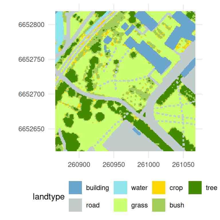
center
Compute landtype_distance
Getting started
Running the function for a station is as follows:
# Compute land type distance to station
landtype_dist <- compute_landtype_distance(stn, landtype_out, f_plot = TRUE)[1] "Process: 18700 - 260966.8/6652718.0 - dtm - 100/1 - path: data/dem"
[1] "Load demo file: data/dem/18700_dtm_25833_d00100m_1.0m.tif"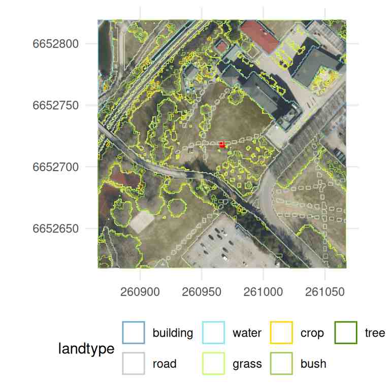
center
Compute class
Getting started
Running the function for a station is as follows:
# Load a digital elevation model
dem <- download_dem_kartverket(stn, name = "dtm")[1] "Process: 18700 - 260966.8/6652718.0 - dtm - 100/1 - path: data/dem"
[1] "Load demo file: data/dem/18700_dtm_25833_d00100m_1.0m.tif"
# Compute maximum horizon
horizon_max <- compute_horizon_max(stn,
step = 0.01)[1] "Process: 18700 - 260966.8/6652718.0 - dtm - 100/1 - path: data/dem"
[1] "Load demo file: data/dem/18700_dtm_25833_d00100m_1.0m.tif"
[1] "Process: 18700 - 260966.8/6652718.0 - dom - 100/1 - path: data/dem"
[1] "Load demo file: data/dem/18700_dom_25833_d00100m_1.0m.tif"
[1] "Process: 18700 - 260966.8/6652718.0 - dtm - 20000/20 - path: data/dem"
[1] "Load demo file: data/dem/18700_dtm_25833_d20000m_20.0m.tif"
Over-riding projection check
Importing raster map <elev>...
   0%   3%   6%   9%  12%  15%  18%  21%  24%  27%  30%  33%  36%  39%  42%  45%  48%  51%  54%  57%  60%  63%  66%  69%  72%  75%  78%  81%  84%  87%  90%  93%  96%  99% 100%
Over-riding projection check
Importing raster map <elev>...
0% 3% 6% 9% 12% 15% 18% 21% 24% 27% 30% 33% 36% 39% 42% 45% 48% 51% 54% 57% 60% 63% 66% 69% 72% 75% 78% 81% 84% 87% 90% 93% 96% 99% 100%Over-riding projection check
Importing raster map <elev>...
0% 3% 6% 9% 12% 15% 18% 21% 24% 27% 30% 33% 36% 39% 42% 45% 48% 51% 54% 57% 60% 63% 66% 69% 72% 75% 78% 81% 84% 87% 90% 93% 96% 99% 100%
# Compute class
class <- compute_class_air_temperature(stn,
                                       landtype_dist,
                                       horizon_max,
                                       dem,
                                       test_type = "WMO",
                                       f_plot = TRUE)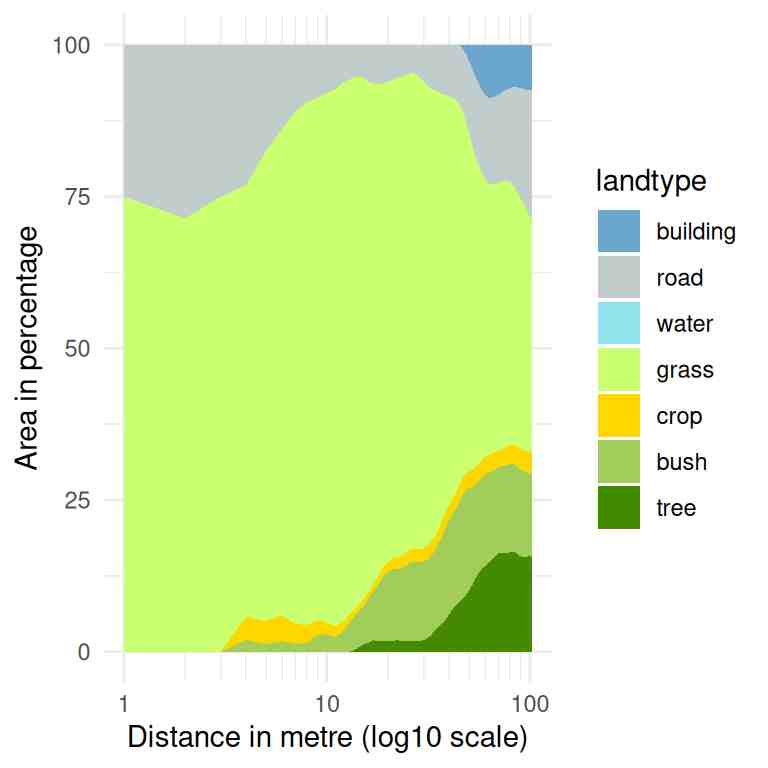
center
[1] " "
[1] "-------------------------------------------"
     class_slope class_vegetation   class_landtype      class_shade
        "class1"         "class1"         "class4"         "class5"
[1] "-------------------------------------------"
[1] "-------------------------------------------"
[1] " "
[1] " "
To compute a class, one need to decide a few input parameters: -
station infos, - landtype classification per distance from the station,
- max horizon derived from DEMs - and whether to use the “MET” or “WMO”
thresholds using test_type,
# Input
land <- landtype_dist
horizon <- horizon_max
dem <- dem
test_type <- "MET"

# Extract column and land type names
colname <- colnames(land)
landtype_name <- colname[-1]
First the area percentage per landtype is computed and then converted into a dataframe for extracting the zones required in the tests (i.e. 3, 5, 10, 30, 100m), including the two rings: 5-10 m and 10-30 m.
# Compute area percentage per land type
df <- land[, colname %in% landtype_name] /
  land[, colname == "total_area"] * 100

# Reshape data.frame, equivalent to pivot_longer()
df <- with(utils::stack(as.data.frame(t(df))),
           data.frame(distance = as.numeric(as.character(ind)),
                      landtype = factor(colnames(df), landtype_name),
                      area = values))

# Compute area within an annular area 5-10m and 10-30m
ring <- land[rownames(land) %in% c(10, 30), colname %in% landtype_name] -
  land[rownames(land) %in% c(5, 10), colname %in% landtype_name]
ring_area <- land[rownames(land) %in% c(10, 30), colname == "total_area"] -
  land[rownames(land) %in% c(5, 10), colname == "total_area"]
ring <- (ring / ring_area) * 100

# Extract areas (%) at 3, 5, 5-10, 10, 10-30, 30, 100m radius for class tests
df_radius <- round(cbind(df[df$distance == 3, "area"],
                         df[df$distance == 5, "area"],
                         ring[rownames(ring) == 10],
                         df[df$distance == 10, "area"],
                         ring[rownames(ring) == 30],
                         df[df$distance == 30, "area"],
                         df[df$distance == 100, "area"]))

# Assign names for rows and columns
rownames(df_radius) <- colname[-1]
colnames(df_radius) <- c("3m", "5m", "5-10m", "10m", "10-30m", "30m", "100m")

df_radius
3m 5m 5-10m 10m 10-30m 30m 100m
building 0 0 0 0 0 0 7
road 25 18 5 8 6 6 21
water 0 0 0 0 0 0 0
grass 75 78 91 87 76 77 39
crop 0 4 1 2 2 2 4
bush 0 1 3 3 14 13 14
tree 0 0 0 0 2 2 16Class per category
Artificial heat
# 1) Sum area percentages of building, road and water (1:3 rows) for each
# distance (columns)
landtypes <- colSums(df_radius[colname[-1] %in%
                                 c("building", "road", "water"), ])
landtypes
3m 5m 5-10m 10m 10-30m 30m 100m
25 18 5 8 6 6 28 Vegetation
# 2) Sum grass to crop area and compute mean over distance classes
vegetation      <- df_radius[colname[-1] %in% c("grass", "crop"), ]
vegetation[2, ] <- colSums(vegetation)
vegetation      <- round(rowMeans(vegetation))
vegetation
grass crop
75 77 Shade
Shade algorithm was recently edited to account for narrow valleys and assign a kinder class as one assumes that the station represents the local environment within 1.5 km.
Otherwise it smoothes out the horizon with an hour time window.
# 3) Projected shade limits
height <- compute_horizon_rollmean(stn, horizon)
# Compute the percentage of terrain within 1500 m to assess if the station
# is in a valley or an open terrain, the threshold being 66.666%
range_valley <- (horizon[, "range"] > 100 & horizon[, "range"] <= 1500)
range_valley_tot <- sum(range_valley) / dim(horizon)[1] * 100
if (range_valley_tot < 66.666){
  # 3.1) if station is in an open terrain, compute the max of the horizon
  # (the default behaviour)
  shade <- max(height)
}else{
  # 3.2) if station is in a deep vally, set heights in the valley to 0 and
  # compute the mean to sill get an evaluation of the close environment
  height[range_valley] <- 0
  shade <- mean(height)
}
names(shade) <- "shade"
shade
shade
53.50798 WMO vs MET class
# Set matrix of class test parameters
if (test_type == "WMO") {
  class_names <- c("class1", "class2", "class3", "class4", "class5")
  type_names  <- c(names(landtypes), names(vegetation),
                   names(shade), names(slope))
  params <- matrix(c(NA, NA, NA,  1,  5, NA, 10, 51,  0,  5, 19,
                     NA, 1,  5,  NA, NA, 10, NA, 51,  0,  7, 19,
                     NA, 5,  NA, 10, NA, NA, NA, 99, 51,  7, 99,
                     30, NA, NA, 50, NA, NA, NA, 99, 99, 20, 99,
                     NA, NA, NA, NA, NA, NA, NA, 99, 99, 99, 99),
                   nrow = length(class_names),
                   ncol = length(type_names),
                   byrow = TRUE,
                   dimnames = list(class_names,
                                   type_names))
} else if (test_type == "MET") {
  class_names <- c("class1", "class2", "class3", "class4", "class5")
  type_names  <- c(names(landtypes), names(vegetation),
                   names(shade), names(slope))
  params <- matrix(c(NA, NA, NA,  1,  5, NA, 10, 51,  0,  7, 19,
                     NA, 1,  5,  NA, NA, 10, NA, 51,  0,  7, 19,
                     NA, 5,  NA, 10, NA, NA, NA, 99, 51,  7, 99,
                     30, NA, NA, 50, NA, NA, NA, 99, 51, 20, 99,
                     NA, NA, NA, NA, NA, NA, NA, 99, 99, 99, 99),
                   nrow = length(class_names),
                   ncol = length(type_names),
                   byrow = TRUE,
                   dimnames = list(class_names,
                                   type_names))
}
params
3m 5m 5-10m 10m 10-30m 30m 100m grass crop shade slope
class1 NA NA NA 1 5 NA 10 51 0 7 19
class2 NA 1 5 NA NA 10 NA 51 0 7 19
class3 NA 5 NA 10 NA NA NA 99 51 7 99
class4 30 NA NA 50 NA NA NA 99 51 20 99
class5 NA NA NA NA NA NA NA 99 99 99 99