Getting started with sitingclass

Getting started with `sitingclass`

The sitingclass package computes the exposure of a weather station. Currently, the package is built for Norwegian weather stations that are maintained by the Norwegian Meteorological Institute (https://www.met.no/).

Check the README for information on this R package’s installation, authentication, dependencies, as well as the source of used data and metadata.

From R, get the following examples by loading the library and running:

vignette("getting_started", package = "sitingclass")

Plot the station with background imagery

Get the station’s metadata

Load the library and extract the metadata for a given station using the Met’s stationid

library(sitingclass)

# Define station ID as used by other functions below
stationid <- 18700

# Get station metadata
stn <- get_metadata_frost(stationid, path = NULL)
# Set default path to NULL in order to print and not save plots

The result is a SpatVector with coordinates in UTM33 (unit: metre) and metadata:

the station: name, coordinates (lat/lon), alternative ids, exposure, organisation,
the physical parameter: name, id, level, sensor, performance,
the processing parameters:
- dx: the radius in metre (default: 1) of the boundary box that defines the area to download
- resx: the spatial resolution in metre (default: 100)for the data to download
- path: where to save the output figures (default: output/stationid)

stn

 class       : SpatVector 
 geometry    : points 
 dimensions  : 1, 26  (geometries, attributes)
 extent      : 260966.8, 260966.8, 6652718, 6652718  (xmin, xmax, ymin, ymax)
 source      : 18700_stn.gpkg
 coord. ref. : ETRS89 / UTM zone 33N (EPSG:25833) 
 names       : level parameterid sensor stationid  elev   lat   lon elev.1
 type        : <int>       <int>  <int>     <int> <num> <num> <num>  <num>
 values      :     0         211      0     18700    94 59.94 10.72     94
    element.name    station.name (and 16 more)
           <chr>           <chr>              
 Air temperature OSLO - BLINDERN

# Reverse dataframe to show last added parameters
rev(as.data.frame(stn))

  resx  dx performance.value       performance.to     performance.from
1    1 100           unknown 9999-01-01T00:00:00Z 1937-01-01T06:00:00Z
  exposure.value          exposure.to        exposure.from           WIGOS
1              1 9999-01-01T00:00:00Z 1931-01-01T06:00:00Z 0-20000-0-01492
     Fast_IP.2             WMO    Fast_IP.1      Fast_IP      organisation.to
1 10.240.10.15 0-20000-0-01492 10.240.10.15 10.240.10.15 0001-01-01T00:00:00Z
     organisation.from organisation.value    station.name    element.name
1 1996-12-01T00:00:00Z             MET.NO OSLO - BLINDERN Air temperature
  elev.1   lon     lat elev stationid sensor parameterid level
1     94 10.72 59.9423   94     18700      0         211     0

Construct a boundary box

From SpatVector

The easiest method is to use the default processing parameters that are contained in the SpatVector. One could edit their values directly during loading of the metadata with: get_metadata_frost(stationid, dx=1, resx=100, path="output/stationid"

box <- make_bbox(stn)
box

SpatExtent : 260866, 261067, 6652618, 6652819 (xmin, xmax, ymin, ymax)

From coordinates

The other method is to manually extract the coordinates from the SpatVector and set manually the radius dx

# Get coordinates
centre <- terra::crds(stn)
centre

            x       y
[1,] 260966.8 6652718

# Define radius
dx <- 100

# Construct box to extract WMS tile
box <- make_bbox(centre, dx = dx)
box

SpatExtent : 260866, 261067, 6652618, 6652819 (xmin, xmax, ymin, ymax)

Plot background tile with station

The boundary box is then used to get background maps from WMS layers, in this case "esri" satellite imagery. The list of all available layers is found in the function documentation.

# Plot ESRI imagery tile
plot_tile_station(stn, box, tile_name = "esri")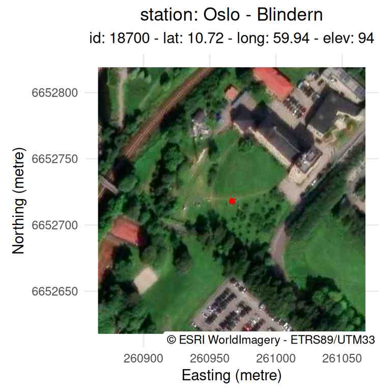

A satellite image with the station location as a red dot.

Plot station, tile and grid

The function plot_station_grid() adds a grid and circles to the image. The grid/circle size and interval are defined by the radius of the image with default 10-m, 50-m, 100-m and 1000-m.

In this example, the tile name "ortofoto" gets aerial imagery from Kartverket, the Norwegian Mapping Authority.

# Plot tile with grid and proximity circles
plot_station_grid(stn, tile_name = "ortophoto_demo", grid_scale = 10)

[1] "grid: ortophoto_demo --- 10-m scale"
[1] "18700_ortophoto_25833_d00016m.tif" "18700_ortophoto_25833_d00016m.tif"
[1] "/home/runner/work/_temp/Library/sitingclass/extdata/18700_ortophoto_25833_d00016m.tif"
[2] "/home/runner/work/_temp/Library/sitingclass/extdata/18700_ortophoto_25833_d00016m.tif"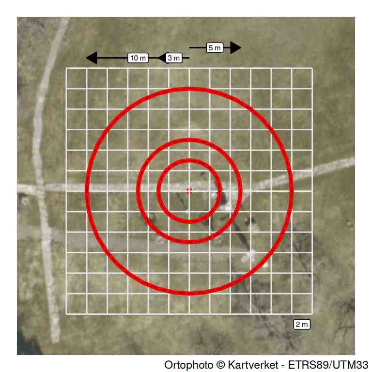

Grid and buffer with ‘Norge i bilder’ imagery.

Plot Digital Elevation Models (DEM)

Download DEMs from Kartverket

The area of the DEM is defined by the boundary box set above in addition to the spatial resolution resx that is required by Kartverket’s Web Coverage Service (WCS).

Two types of models are available:

DTM: Digital Terrain Model that represents the ground elevation ("dtm" in Norwegian)
DSM: Digital Surface Model that represents the surface elevation including trees and buildings ("dom" in Norwegian)

The function fetches already downloaded and stored locally DTMs if the flag f_overwrite is set to FALSE, otherwise it overwrites the file, the default behaviour.

f_ow  <- FALSE
dem   <- download_dem_kartverket(stn,
                                 name = "dtm",
                                 f_overwrite = f_ow)
dsm   <- download_dem_kartverket(stn,
                                 name = "dom",
                                 f_overwrite = f_ow)

Plot DEMs with `rayshader`

The package rayshader is used here to produce 2D and 3D visualisations of the DEMs with shaded relief. Here is an example where the 100-m DSM raster is converted to a matrix and then plotted with a shaded relief.

library(rayshader)
elmat   <- raster_to_matrix(dsm)
elmat %>%
  sphere_shade(texture = "desert") %>%
  plot_map()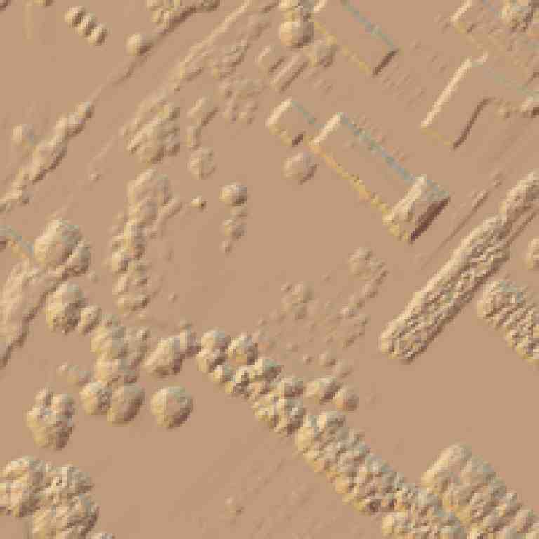

Hillshade of the 100-m digital surface model.

Example for larger areas

For larger areas, one can also set the boundary box manually in download_dem_kartverket() with stn being the centre, dx the radius of the boundary box and resx the horizontal resolution of the model. In this example, a 20-km radius, 20-m resolution DEM is downloaded and plotted.

demkm <- download_dem_kartverket(stn,
                                 name = "dtm",
                                 dx = 20e3,
                                 resx = 20,
                                 f_overwrite = f_ow)
elmatkm <- raster_to_matrix(demkm)
elmatkm %>%
  sphere_shade(texture = "desert") %>%
  plot_map()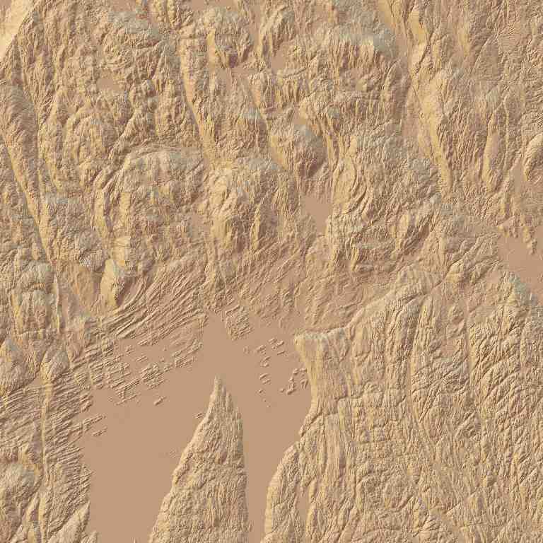

Hillshade of the 20-km digital elevation model.

Plot a sun diagram

The function plot_station_horizon_sun() computes and plots sun diagram from the following inputs:

the station location (stn)
a local and regional Digital Elevation Model (dem and demkm) to show shading from the landscape
a local Digital Surface Model (dsm) to show shading from local buildings or trees.

plot_station_horizon_sun(stn)

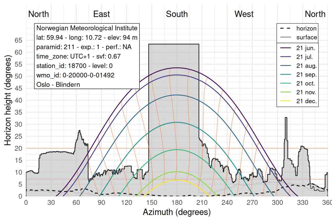
Horizon and sun diagram for the station 18700

Compute the final siting class

The function plot_station_siting_context() eventually contains a workflow producing the figures necessary for station inspections and estimate the final siting class:

Gets the metadata of a Met weather station
Plot station with grid and circles covering the area with the radii 10-m, 50-m, 100-m, 1000-m
Plot the sun diagram
Compute the siting class of the station

# Set timezone to avoid time shift between winter and summer time
Sys.setenv(TZ = "UTC") # "Europe/Oslo"

# The main function plotting sun diagram and context for a weather station
plot_station_siting_context(stationid = 18700,
                            paramid = 211,
                            f_verbose = FALSE,
                            f_pdf = FALSE)

Pierre-Marie Lefeuvre

2025-04-22